Must know Advanced Functions and Formulas in Excel

Microsoft Excel is one special name among many software, which is very popular, and used in many different industries, for various applications. The application is used for some very basic tasks (accounting, data entry, etc) and even for very complex tasks (data analysis, data visualization, etc).

So, it becomes a must-have skill to have a competitive edge in the job market. The thing is that Excel has many concepts, so it might seem overwhelming to learn and understand so many concepts and implement them. Especially when it comes to functions in MS Excel, there are around 450+ functions, so clearly, it becomes too much to digest.

Advanced Functions and Formulas in Excel

But when it comes to advanced Excel functions, there are some functions you must be familiar with, so that you can use them as and when required. So, in this article, we are going to learn about some Advanced functions and formulas in Excel, which you must know about.

What is Advanced Excel?

You might have heard the term “Advanced Excel” quite a few times now, but if you are confused about what is it actually, let’s have a quick look at what Advanced Excel is. Actually when you say “Advanced Excel”, you are referring to a higher level of proficiency and expertise in using the Microsoft Excel Software beyond the basic functionalities.

Understanding Advanced Excel allows us to perform complex tasks, like data analysis, data visualization, and more. Here is some of the stuff associated with Advanced Excel –

• Advanced (complex) functions and formulas
• Data Analysis Techniques (This includes PivotTables, Power Query, etc)
• Data Visualization and Dashboard Creation.
• VBA and Macros.
• Data Validation.

There might be some more things related to Advanced Excel, but these are some of the frequently used ones, with which you should be familiar, and having good knowledge related to these can bring out a lot of opportunities for you in the job market.

Advanced Functions in Excel

Now we are going to head toward a discussion about some advanced functions and formulas in MS Excel, which you must be familiar with. First of all, let’s have a look at a quick list of the functions that we are going to discuss, and then quickly we will turn towards discussing each one separately. Here’s the list –

Function Name	Description
VLOOKUP Function	Searches for a value in a table and returns a corresponding value.
INDEX / MATCH Function	Retrieves a value at the intersection of a specified row and column.
XLOOKUP Function	Finds and retrieves values in a range or array.
SUMIF/SUMIFS Function	Adds values based on a single or multiple criteria.
COUNTIF/COUNTIFS Function	Counts cells based on specified criteria.
UNIQUE Function	Returns a list of unique values from a range or array.
LEFT/MID/RIGHT Functions	Extracts characters from a text string based on their positions.
IF Function	Performs conditional evaluations and returns values based on a specified condition.
CONCATENATE Function	Joins multiple strings into a single string.
TRIM Function	Removes extra spaces from a text string.

As you can see, there are quite a lot of functions in the above list, that we need to discuss, so now, let’s get right into it.

VLOOKUP function

VLOOKUP is used very much in Excel, thanks to the simplicity it provides. As the name of this function says, VLOOKUP means Vertical Lookup, which means that we are searching for a value in the first column of the table, and then retrieve the corresponding value in the same row, from another specified column.

So, as the definition says, this function is widely used for data lookup purposes in Excel. Let’s have a quick look at an example, which should give a better idea.

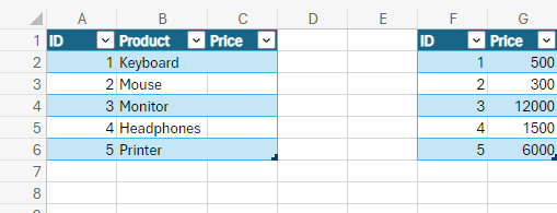
From the above image, you can look at the data that we have. We have two tables, in which we have some product-related data. In the first table, we have the ID and product name, and a column for the price, in which, data needs to be filled. Another table has IDs for the same products and Prices.

Now let’s say that we need to look for the price, in this case, we can make use of the VLOOKUP function. Here is the basic syntax of the VLOOKUP function –

=VLOOKUP(lookup_value, table_array, col_index_num, [range_lookup])

Here are the explained parameters for the VLOOKUP function –

• lookup_value: The value you are looking for.
• table_array: Need to provide the table range from which the data is to be retrieved.
• col_index_num: column number from which the corresponding value is to be retrieved.
• [range_lookup]: This parameter is optional and is a logical value. TRUE for approximate match, FALSE for exact match.

For our above example, here is what the VLOOKUP function looks like –

=VLOOKUP(Table1[@ID], Table2[#All], 2, FALSE)

This function is supposed to be put in the C2 cell, and you would find that the price comes there. You may try the VLOOKUP function from the above example, and understand the implementation of the VLOOKUP function.

INDEX / MATCH function

The INDEX Function, and the MATCH Function when used together, are used for lookup purposes. When XLOOKUP wasn’t there, many people used INDEX and MATCH functions together, because they handled the drawbacks of VLOOKUP, for VLOOKUP, the lookup value must be in the first column for it to work correctly.

But then, INDEX and MATCH together were used in the lookup. Here is how you can use it. We will use the same example to understand INDEX and MATCH Functions because we are doing the same things, but before that, let’s understand the syntax of both functions –

=INDEX(array, row_num, [column_num])

• array: range of cells.
• row_num: The row number from which the value needs to be returned. If this is omitted, then the column_num is required.
• [column_num]: The column number from which the value is to be returned. If omitted, then row_num is required.

=MATCH(lookup_value, lookup_array, [match_type])

• lookup_value: Value used to find another required value.
• lookup_array: Array of values.
• [match_type]: This specifies the type of match. It can have values as 0, 1, and -1. 0 means Exact match, 1 means the largest value less than or equal to the lookup value, and -1 means finding the smallest value greater than or equal to the lookup value.

So, let’s see how we use the INDEX and MATCH Functions together for lookup purposes –

=INDEX(Table2[Price], MATCH([@ID],Table2[ID], 0))

So, using the above function in cell C2 would get you to the answer. So, this is how to make use of the INDEX and MATCH functions, as an alternative to VLOOKUP, to overcome the drawbacks of VLOOKUP. But now, XLOOKUP has come to overcome the drawbacks of VLOOKUP.

XLOOKUP

XLOOKUP has come to overcome the drawbacks of VLOOKUP. While VLOOKUP is simple to use, which is why it’s used a lot, it has some drawbacks, which creates the need for XLOOKUP. XLOOKUP is available in the latest versions of MS Excel, and not in MS Excel 2016 and 2019. XLOOKUP is used to find things in the table or a range by row.

Let’s understand the XLOOKUP function with the help of the same example as we saw in VLOOKUP, but just XLOOKUP makes it more simple. The situation is the same. In this case, as well, we just need to look for the marks of a student from his/her ID.

First of all, here is the syntax for the XLOOKUP function –

=XLOOKUP(lookup_value, lookup_array, return_array, [if_not_found], [match_mode], [search_mode])

• lookup_value: The value to search for.
• lookup_array: array or range to search from.
• return_array: The array or range to return.
• [if_not_found]: This is optional and is the value to be returned if no match is found.
• [match_mode]: Specifies how to match lookup_value against the values in the lookup array. This is an optional parameter.
  • 0 for an exact match, and an error if not found. (default value)
  • -1 for an exact match, and if none is found, return the next smaller item.
  • 1 for an exact match, and if none is found, return the next larger item.
  • 2 for a wildcard match, where * and ? have special meaning.
• [search_mode]: Specifies the search mode to use. This parameter is optional.
  • 1 for search starting from the first item. (default value)
  • -1 for performing a search from the reverse.
  • 2 for performing a binary search(lookup_array should be sorted in ascending order)
  • -2 for performing a binary search(for lookup_array sorted in descending order)

In our case, the XLOOKUP function looks something like this –

=XLOOKUP([@ID], Table2[ID], Table2[Price], 0)

As you can see, we gave the lookup value, lookup array, and the return array, and we got the corresponding value, which we wanted to lookup. This overcomes the drawbacks of VLOOKUP and is very useful. The last 0 that we are passing is for [if_not_found], which means that if the match was not found, return 0.

You can try the XLOOKUP function on the above-specified example of VLOOKUP.

SUMIF and SUMIFS Function

If you are familiar with MS Excel already, you must be familiar with the simple SUM function, which is simply used to sum from the given range. It is very simple, and straightforward, because we just need to provide the range to the SUM function, and we are done.

But sometimes, we might need to do the sum according to some conditions. Let’s take an example to better understand this situation.

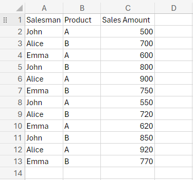
Let’s say that we have this data as mentioned below. It has the names of the salesperson, the product sold, and the price. Now let’s say that we want to calculate how much sales John has made, in this case, we need to do the sum, but this time it’s conditional. This is where the function SUMIF comes into action, and simply if there are multiple conditions, we use the SUMIFS function.

Here is what the data looks like –

So here, let’s first try to use the SUMIF function to know how much sales were made by John. For this, we just need to sum the prices, where the salesperson is John. This is how you do it using the SUMIF function. First of all, let’s have a look at the syntax of the SUMIF function –

=SUMIF(range, criteria, [sum_range])

• range: Range of cells that you want to evaluate with criteria.
• criteria: This defines which cells will be added.
• [sum_range]: This defines the actual cells to be added. This parameter is optional, and if omitted, the cells in the range argument are added.

Now it’s time to apply the function to the above example, to get the desired output. Here is the function, that you can also copy and apply.

=SUMIF(A2:A13, “John”, C2:C13)

The first argument we are passing is the range(which is the salesperson), and the second argument specifies “John”, which is the criteria, and then we are specifying the range to sum.

Now that we have understood the SUMIF function, we can easily understand the SUMIFS function. You might have spotted that when we are using the SUMIF function, we are giving only one criterion, but what if we have multiple conditions to sum? Like for example, if we want to know the number of sales done by John from the above data, we can do it easily using SUMIF, but if we want to know the amount of sales done by John by selling “product A”, this is something where you would need SUMIFS function. So, let’s try this example –

First of all, here is the syntax of the SUMIFS function –

SUMIFS(sum_range, criteria_range1, criteria1 …)

As you can see, you just need to give the sum_range, then you need to provide the criteria_range and criteria(so you can also provide multiple criteria ranges and the criteria). So, for our above example, the function becomes something like this –

=SUMIFS(C2:C13, A2:A13, “John”, B2:B13, “A”)

As you can see, the sum range was given first, and then we gave two criteria ranges and their criteria. I hope you can understand the SUMIF and SUMIFS functions, and also understand how to use them.

COUNTIF and COUNTIFS Function –

With your Excel basics knowledge, you might be familiar with the good old COUNT function, which is very useful, and very basic. It does what its name says, counting the cells with numbers in the given range. This is all straightforward, but sometimes, you might need to count values based on some condition, and this is when you would be required to use the COUNTIF and COUNTIFS functions.

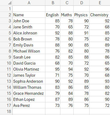
Let’s get this from an example – let’s say that you have data on student’s marks, for different subjects, like Maths, Physics, Chemistry, and English. Let’s say you want to count the number of students who got more than 80 marks in Chemistry. This is where you would use the COUNTIF function. Let’s have the data – it looks something like this –

Now, let’s say that we need to count the number of students who got more than 80 marks in Chemistry. So, for that reason, we need to use the COUNTIF function, which has the following syntax –

=COUNTIF(range, criteria)

• range: range of cells from which you want to count.
• criteria: a condition that tells which cells are to be counted.

So, in our case, the range would be the cells that contain chemistry marks, and the criteria would be that the marks should be greater than 80. Here is the actual formula to be used –

=COUNTIF(E3:E17, “>80”)

The above formula is for counting how many students got more than 80 marks in Chemistry. Please consider changing the range according to the data that you have placed in your Excel sheet, to get the correct output.

Now that we have understood the COUNTIF function, it has become easy for us to understand the COUNTIFS function. When we had just one criterion, we used the COUNTIF function, and if in any case, we have more than one criterion, like greater than 80 marks in Chemistry, and greater than 85 marks in Maths together, then we need to make use of the COUNTIFS function.

Here is the syntax for the COUNTIFS function –

=COUNTIFS(criteria_range1, criteria, …)

As you can see, to the COUNTIFS function, we are just providing the criteria range and criteria, and we should be comfortable getting to the output. Here is the actual formula for getting the count of students, who scored more than 80 marks in Chemistry, and more than 85 in Maths.

=COUNTIFS(E3:E17, “>80”, C3:C17, “>85”)

As you can see, we have provided two criteria ranges and criteria, and we get the number of valid students. So, I hope you understand the concept of COUNTIF and COUNTIFS function. You can try the examples, to understand them better, and be practical.

UNIQUE Function

Now we are going to discuss an interesting function in MS Excel, which is the UNIQUE function. The thing is that this function is not available in the Excel versions of 2019, or even earlier, so to be able to use this function, you need to have Excel 365, and Excel 2021, or even you can use it on Excel for the web(it’s free).

As the name says, the UNIQUE function returns a list of unique values from the given list or range. It’s as simple as that. So, let’s just try this once with an example, to understand it better.

First of all, here is the syntax of the UNIQUE function –

=UNIQUE(array, [by_col], [exactly_once])

• array: range or array from which unique rows or columns need to be returned.
• [by_col]: if False(or omitted), it compares the rows against each other and returns the unique rows. If True, compare the columns against each other, and return the unique columns. (Optional Parameter)
• [exactly_once]: If True, return rows or columns that occur exactly once from the array. If False(or omitted), return all the distinct rows or columns from the array. (Optional Parameter)

Let’s say that we have a list of some names, and we need to get the unique names only. Here, the UNIQUE function can help us. Here is what the data looks like. There are a lot of rows, so we are showing only a few first rows to get an idea of the data.

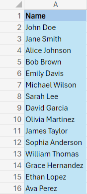
So, here is the UNIQUE function being used to get the unique values from the given list or array. You can also try to use this function so that you can get comfortable with this function. Remember that as of now, to be able to use the UNIQUE function, you need Excel 365, or Excel 2021, or you can use it on Excel for the web.

LEFT, MID, RIGHT Functions

In Excel, there are many Text-based functions, which are used to do some different things, like converting text to lowercase, or uppercase, getting the length of the text, and much more. Here, we are going to discuss three very important functions among these text functions, which are LEFT, MID, and RIGHT functions.

Although we are discussing these functions together, you don’t need to use these functions together, but in one example frame, we are going to discuss them all.

So, let’s consider an example, where we have the registration number of a student, which is a combination of three things, for example, 2025CSE101 is a registration number, and it’s a combination of three things, like year of admission, branch(CSE), and the roll number. We need to extract this information in separate columns. Here is how LEFT, MID and RIGHT function come into the picture.

First of all, let’s have a look at the data that we have got –

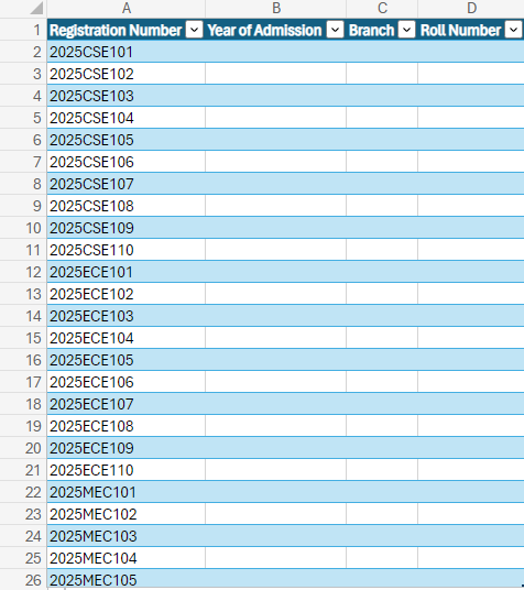
So, as you can see, we have the Registration number, from which, we need to extract the information like year of admission, Branch, and Roll number. For this, we can make use of these functions – LEFT, MID, and RIGHT.

First of all, let’s take a look at the LEFT function. As the name says, it is used to return the first character or specified number of characters from the start of the string. For example, in our case, we can extract the year of admission as the first 4 characters from the registration number. Here is the syntax for the LEFT function –

=LEFT(text, [num_chars])

• text: The text string containing the characters you want to extract.
• [num_chars]: Specifies how many characters to extract. This parameter is optional and has a value of 1 if omitted.
  So, here is the LEFT Function in our case –

=LEFT([@[Registration Number]], 4)

Actually, we have the data in the table, and we are first providing the text, and then we are providing the number of characters. If you try to apply the above function, you will get the required year of admission.

Next comes the Branch which we need to extract, and for this, we can make use of the MID function. As the name says, this MID function helps us get the characters from the middle of the string, from the given starting position to the given length. Let’s have a look at the syntax of the MID function.

=MID(text, start_num, num_chars)

• text: Text from which you want to extract the characters.
• start_num: position of first character to extract.(starting from 1)
• num_chars: number of characters to extract.

Here is what the function looks like in our case –

=MID([@[Registration Number]], 5, 3)

As you can see, we are providing the registration number, then we are providing that the first character position is 5, and from that, we need to extract 3 characters. You may try to use this function in your table as well, but please take into account some obvious things, like table info.

The last thing that we want to do here, is to extract the roll number, which is to the right. We may use MID for it as well, saying that our first character is in the 8 position, and from there, we need 3 characters, but even better than that, you may use RIGHT. As the name says, the RIGHT function is used to return the specified number of characters from the end of the string. Here is the syntax for the RIGHT function –

=RIGHT(text, [num_chars])

• text: the text from which you want to extract the characters.
• [num_chars]: Specifies how many characters to extract. An optional parameter, and if omitted, the value is 1.

As you can see, we have the RIGHT function syntax, and here is the actual function that we are going to use –

=RIGHT([@[Registration Number]], 3)

As you can see, we have given the registration number, and have asked for 3 characters from the last.

IF Function

In Excel, at times, we need to do something based on some condition, This should be clear with an example – let’s say that we have some data in Excel, where there are names of some students, and then there are marks of students. Now, we need to check if the student has passed or failed. This is where the IF function can be used.

First of all, let’s have a look at the syntax of the IF Function –

=IF(logical_test, [value_if_true], [value_if_false])

• logical_test: This is the value or expression which can be evaluated as TRUE or FALSE.
• [value_if_true]: Value returned if the logical test is True. If omitted, the value returned is TRUE.
• [value_if_false]: The value returned if the logical test is FALSE. If omitted, FALSE is returned.

As you can see, we now have the syntax of the IF function with us. Now let’s have a look at an example, which provides more clarity about the IF function.

Let’s say that we have the names of students and their marks out of 100. We need to fill another column, where we are going to write pass or Fail, according to the condition. Here is what the data looks like –

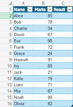
As you can see, we have the marks with us, but right now, we just need to add the result, as Pass or Fail, according to the marks. So the rule says that if marks > 35, the student is passed, otherwise the student fails. Here is the actual IF function that we are going to use here –

=IF([@[ Marks]]>35, “Pass”, “Fail”)

We have the data formatted as a table, and we are checking if the marks are greater than 35, if the expression is True, then we return Pass, otherwise, we return Fail. So, I hope that you can understand the IF function. The IF function can also be used in complex situations, like nesting of IF functions, but we have discussed the core idea of the IF Function.

CONCATENATE

One more interesting function that we are going to talk about right now, is the CONCATENATE function. As the name says, it helps to join two or more text strings into one string. We might need to use the CONCATENATE function at times, whenever we are required to concatenate strings.

Let’s have a look at an example, through which we can understand the CONCATENATE function easily.

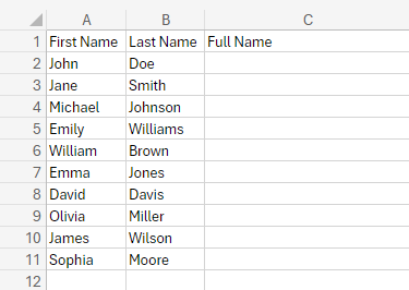
In the below example, we have the first name and last name, and the task here is to concatenate the first name and last name, to make up the full name.

This is so simple. Let’s have a look at an example, which makes us more comfortable with understanding the CONCATENATE function. First of all, here is the syntax of the CONCATENATE function –

=CONCATENATE(text1, [text2], …)

We need to give it the text, which is going to be concatenated. Let’s have a look at the actual function, which we are going to use.

=CONCATENATE(A2, ” “, B2)

As you can see, we have got the concatenate function, which you can easily use. You can practice this function on several text options so that you become comfortable with the concatenate function.

TRIM Function

Now let’s have a look at the TRIM Function, which is used to remove the extra spaces from the text, only leaving a single space between words. This function can be understood with the help of a simple example. Here is the data for the same –

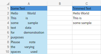
As you can see in the text in the data, there is some extra space, that we don’t need, so to get rid of that extra space, we can make use of the TRIM Function. It comes so handy, that you can use it anytime on the text. Here is the syntax for TRIM –

=TRIM(text)

Let’s have a look at the actual formula that we are going to use.

=TRIM(A2)

So, due to the above function, you would see that the text from the A2 cell gets its spaces removed, and is inserted in the specified cell.

Conclusion

Here, we have explored some of the Advanced Excel functions, which you must know about. There are around 450+ functions in Excel, and it becomes very hard to remember all or most of the functions. But the thing is that there are some functions that you would use more frequently than the others.

This tutorial introduced you to several Advanced Functions that you must be familiar with. I hope that you can understand all the discussed functions here, and could understand their implementation.

FAQs related to Advanced Functions in Excel